Practical Historical Value-at-Risk

In this article, I'll walk through the steps to calculate a 95% 1-day Historical VaR for a hypothetical BTC + ETH portfolio. Use the VaR code on Github to calculate your own portfolio VaR!

I helped set up a historical VaR calculation process at an asset manager in South Africa, this is when it really started making sense for me. Previously I've only come across it academically.

I think VaR is an important concept to understand for your own portfolio's risk analysis. Even though this example focuses on cryptocurrency, the methodology can be applied to any set of assets you're interested in, like stocks, bonds, etc.

Any questions? Reach out on LinkedIn or Telegram.

What is VaR and why use it?

It's a single metric that tries to summarise your overall portfolio risk. The same technique can be used on individual assets to give an idea of single-asset risk exposure, but you should look at your combined portfolio to take into account diversification effects. More info at Investopedia VaR

It's useful to understand the value variance your portfolio is exposed to, over a given time horizon, with a certain level of confidence (e.g. 95% confident that you won't lose more than X amount in a day).

It helps you make decisions about how much risk you are willing to take on and whether or not you need to adjust your investment strategy.

This technique can be extended to perform "Stress Testing" scenarios as well. For example, you could calculate the VaR under different market conditions (e.g. a 10% drop in BTC price), or recreate the 2008 financial crisis scenario and see if your portfolio could survive it.

How to calculate Historical VaR

You need historical price data for each asset, this should be transformed to show delta movements, corresponding to the VaR timewindow you're calculating. Kraken provides historical data for various time intervals here.

We'll only need the XBTUSD_60.csv and ETHUSD_60.csv files from the downloaded OHLCV data. If you want to use more recent data, you'll have to extend this dataset yourself.

Step 1: Import historical prices and merge them into one dataframe.

# Read CSV files into polars dataframes
btc_df = pl.read_csv("XBTUSD_60.csv", has_header=False, new_columns=["Timestamp", "BTC_Open", "BTC_High", "BTC_Low", "BTC_Close", "BTC_Volume", "BTC_TradeCount"])
eth_df = pl.read_csv("ETHUSD_60.csv", has_header=False, new_columns=["Timestamp", "ETH_Open", "ETH_High", "ETH_Low", "ETH_Close", "ETH_Volume", "ETH_TradeCount"])

# Ensure both dataframes have Timestamp as Int64
btc_df = btc_df.with_columns(pl.col("Timestamp").cast(pl.Int64))
eth_df = eth_df.with_columns(pl.col("Timestamp").cast(pl.Int64))

# Sort both dataframes by Timestamp
btc_df = btc_df.sort("Timestamp")
eth_df = eth_df.sort("Timestamp")

# Merge the dataframes on Timestamp
merged_df = btc_df.join(eth_df, on="Timestamp", how="outer")
# Remove rows where Timestamp is null
merged_df = merged_df.filter(pl.col("Timestamp").is_not_null())

# Sort the merged dataframe by Timestamp
merged_df = merged_df.sort("Timestamp")

# Fill missing values with the previous value for all columns except Timestamp
columns_to_fill = [col for col in merged_df.columns if col != "Timestamp"]
merged_df = merged_df.with_columns([
    pl.col(col).forward_fill().backward_fill() for col in columns_to_fill
])

# Filter data after 2017 for both BTC and ETH
start_timestamp = int(datetime(2018, 1, 1).timestamp())
merged_df = merged_df.filter(pl.col("Timestamp") >= start_timestamp)

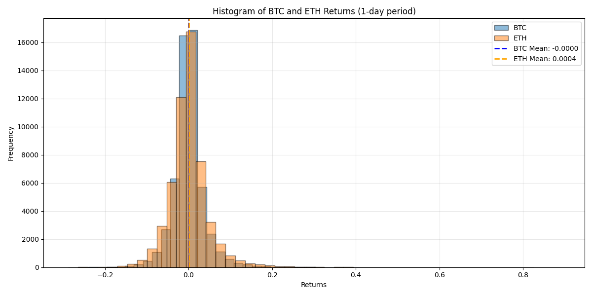
Step 2: Calculate market data delta scenarios for each period (1 day vs 60min in the dataset).

# Calculate the natural log of the ratio of previous Close to current Close
# Looking at a 1-day period (24 hours)
merged_df = merged_df.with_columns([
    (pl.col("BTC_Close").shift(24) / pl.col("BTC_Close")).log().alias("BTC_LogRatio"),
    (pl.col("ETH_Close").shift(24) / pl.col("ETH_Close")).log().alias("ETH_LogRatio")
])
# Remove records where BTC_LogRatio or ETH_LogRatio is null
merged_df = merged_df.filter(
    (pl.col("BTC_LogRatio").is_not_null()) & 
    (pl.col("ETH_LogRatio").is_not_null())
)

# Convert Timestamp to datetime for easier handling
merged_df = merged_df.with_columns([pl.col("Timestamp").cast(pl.Datetime).alias("DateTime")])

Step 3: Exploratory analysis

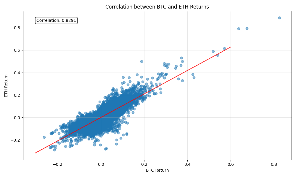
This will show you how strongly correlated "digital assets" are.

Step 4: Calculate the portfolio value at risk.

Market data: (using CCXT to fetch last traded prices from Binance)

• Current BTC price: $ 55,224.48
• Current ETH price: $ 2,315.76

We will consider 2 hypothetical portfolios to compare the impact a riskier asset has on VaR.

• "Balanced Portfolio":

  • 50% BTC: ~0.905395 BTC = $ 50,000.00
  • 50% ETH: ~21.59118 ETH = $ 50,000.00
  • Total portfolio value: $ 100,000.00

• "ETH Weighted Portfolio":

  • 30% BTC: 0.543237 BTC = $ 50,000.00
  • 70% ETH: 30.227657 ETH = $ 50,000.00
  • Total portfolio value: $ 100,000.00

# Apply each of the log ratio returns to the current portfolio value
portfolio_values = []

for row in merged_df.iter_rows(named=True):
    btc_return = math.exp(row['BTC_LogRatio']) - 1
    eth_return = math.exp(row['ETH_LogRatio']) - 1
    new_btc_value = btc_value * (1 + btc_return)
    new_eth_value = eth_value * (1 + eth_return)
    new_total_value = new_btc_value + new_eth_value
    portfolio_values.append(new_total_value)

# Convert the portfolio values to a Polars Series
portfolio_values_series = pl.Series("Portfolio_Values", portfolio_values)

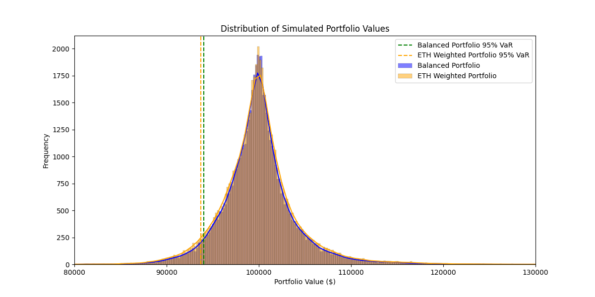
Plotting the portfolio values and finding VaR:

• Balanced Portfolio:

  • 95% VaR (Balanced Portfolio): $ 5,952.21 (5.95% of current portfolio value)
  • This can be interpreted as: With a 95% confidence level, the portfolio will not lose more than $ 5,952 in market value at the end of the next trading day.

• ETH Weighted Portfolio:

  • 95% VaR (Reweighted Portfolio): $ 6,316.73 (6.32% of original portfolio value)
  • This can be interpreted as: With a 95% confidence level, the portfolio will not lose more than $ 6,316 in market value at the end of the next trading day.

From this it's clear how the extra weighting of ETH has increased the VaR risk metric, as expected, compared to the balanced portfolio.

Limitations

• The VaR Calulator only uses market scenarios based on historical data between Jan-2018 and Dec-2023.
• If you want to support additional assets, you'll have to source the extra market data for this.
• If you want to include the latest market data in the calculation, you'll have to do some additional data processing.

Useful links

• Investopedia VaR
• Polars (for fast, performant DataFrames - instead of Pandas)
• CCXT for cryptocurrency data

Keywords

#VaR #ValueAtRisk #PortfolioManagement #Cryptocurrency #Kraken #HistoricalData #Python #CCXT